I had a look at internet and there seem to be R packages for plotting genomic data: GenomeGraphs, ggbio, Sushi.
GenomeGraphs seems to take information directly from Ensembl, which is not my case. Had a try with ggbio with custome annotation (gff):
1
2
3
4
5
6
|
library(ggbio)
library(GenomicRanges)
library(rtracklayer) # imports gff/bed/wig
gff2<-import("~/Desktop/test.gtf") # contains gene/mRNA/exon/CDS
rg2<-GRanges("SM_V7_1", IRanges(4703829,4812964))
autoplot(gff2,which=rg2)
|
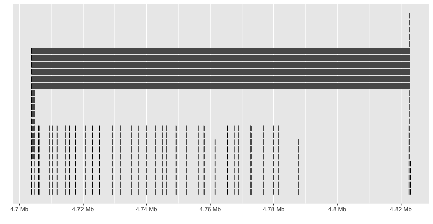
ggbio doesn’t seem to recognize the hierarchy and plots everything. And the labels are missing.
Sushi also seems useful, especially with the plotGenes function, use the example provided:
 1
 2
 3
 4
 5
 6
 7
 8
 9
10
11
12
13
|
library(Sushi)
data(Sushi_genes.bed)

chrom            = "chr15"
chromstart       = 72998000
chromend         = 73020000
chrom_biomart    = 15

plotGenes(Sushi_genes.bed,chrom_biomart,chromstart,chromend ,types=Sushi_genes.bed$type,
     maxrows=1,height=0.5,plotgenetype="arrow",bentline=FALSE,col="blue",
     labeloffset=1,fontsize=1.2)

labelgenome(chrom, chromstart,chromend,side=1,scipen=20,n=3,scale="Mb",line=.18,chromline=.5,scaleline=0.5)
|
Resulted in the same figure.
The only thing is that I will need a bed file with information like:
1
2
3
4
|
 chrom    start     stop  gene score strand
 chr15 73017309 73017438 COX5A     .     -1
 chr15 72999672 72999836 COX5A     .     -1
 chr15 73003042 73003164 COX5A     .     -1
|
So transformed gff to bed:
1
|
grep Smp_322290 Sm_V7_r12.gff| grep CDS |sed 's/;/ /'| awk '{print $1 "\t" $4 "\t" $5 "\t" $10 "\t" "." "\t" $7}'|sed 's/Parent=//'
|
1
|
bdata<-read.delim("~/Desktop/test.bed", sep=" ", header = T)
|
a custome bed file:
 1
 2
 3
 4
 5
 6
 7
 8
 9
10
11
12
13
14
15
16
17
18
19
20
21
22
23
24
25
26
27
28
29
30
31
32
|
chrom start stop gene score strand type
SM_V7_1 33135620 33135696 Smp_012860.1 . 1 CDS
SM_V7_1 33135730 33135847 Smp_012860.1 . 1 CDS
SM_V7_1 33135886 33136029 Smp_012860.1 . 1 CDS
SM_V7_1 33136062 33136237 Smp_012860.1 . 1 CDS
SM_V7_1 33137617 33137839 Smp_012860.1 . 1 CDS
SM_V7_1 33139243 33139362 Smp_012860.1 . 1 CDS
SM_V7_1 33140579 33140630 Smp_012860.1 . 1 CDS
SM_V7_1 33141423 33141616 Smp_012860.1 . 1 CDS
SM_V7_1 33142706 33142927 Smp_012860.1 . 1 CDS
SM_V7_1 33134853 33135619 Smp_012860.1 . 1 utr
SM_V7_1 33142926 33143037 Smp_012860.1 . 1 utr
SM_V7_1 33134851 33135030 Smp_012860.2 . 1 CDS
SM_V7_1 33136062 33136237 Smp_012860.2 . 1 CDS
SM_V7_1 33137617 33137839 Smp_012860.2 . 1 CDS
SM_V7_1 33139243 33139362 Smp_012860.2 . 1 CDS
SM_V7_1 33140579 33140630 Smp_012860.2 . 1 CDS
SM_V7_1 33141423 33141616 Smp_012860.2 . 1 CDS
SM_V7_1 33142706 33142927 Smp_012860.2 . 1 CDS
SM_V7_1 33134803 33134850 Smp_012860.2 . 1 utr
SM_V7_1 33142926 33143037 Smp_012860.2 . 1 utr
SM_V7_1 33135620 33135696 g789.t1 . 1 CDS
SM_V7_1 33135730 33135847 g789.t1 . 1 CDS
SM_V7_1 33135886 33136029 g789.t1 . 1 CDS
SM_V7_1 33136062 33136237 g789.t1 . 1 CDS
SM_V7_1 33137617 33137839 g789.t1 . 1 CDS
SM_V7_1 33139243 33139362 g789.t1 . 1 CDS
SM_V7_1 33140579 33140630 g789.t1 . 1 CDS
SM_V7_1 33141423 33141616 g789.t1 . 1 CDS
SM_V7_1 33142706 33142927 g789.t1 . 1 CDS
SM_V7_1 33134853 33135619 g789.t1 . 1 utr
SM_V7_1 33142926 33143037 g789.t1 . 1 utr
|
With the following command:
1
|
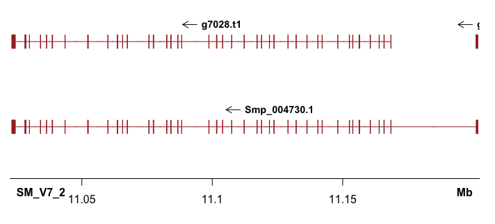
plotGenes(bdata, chrom=chrom,chromstart = chromstart,chromend = chromend, types=bdata$type, maxrows=50,bheight=0.08,plotgenetype="box",bentline=FALSE,col="brown", labeloffset=.2,fontsize=0.9,arrowlength = 0.025,labeltext=TRUE)
|
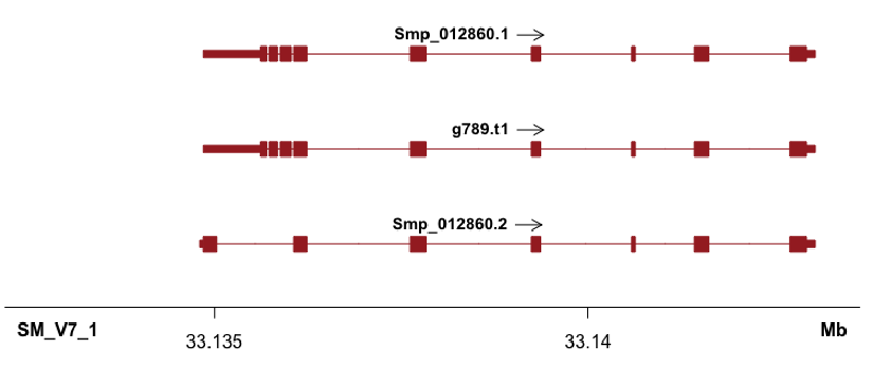
Shown in the title figure. It’s nice that the UTR (shorter than cds/exon), as well as multiple annotations can also plotted (what I need!).
It’s always good to pre-filter your annotation file as two many lines will slow down the plotting process. I have a bed file with 6400 lines and it processes quickly.
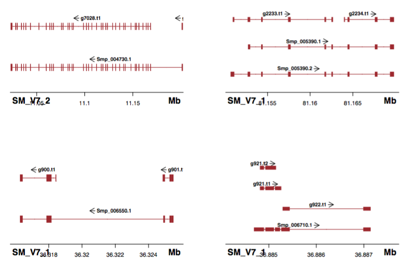
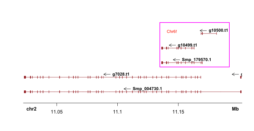
But there seems a bug that Sushi will plot genes in the start-end coordinates from all chromosomes (although you had defined “chrom”; I tried to upgrade to the latest version (1.7.1) but still not solved).
As Mike Smith pointed out on Bioconductor, it’s better to subsetting the bed file before plotting:
bed.sub <- bed[ which(bed[,"chrom"] == 6 & bed[,"start"] >= 132647962 & bed[,"end"] <= 132947962),]
plotGenes(bed.sub)
But this will also cause an error:
1
2
|
 Error in FUN(X[[i]], ...) :
  only defined on a data frame with all numeric variables
|
Have to save bed.sub to a new file and read it into R, then everything fine:
1
2
3
4
5
|
bed.sub <- bed[which(bed[,"chrom"] == chr & bed[,"start"] >= chrstart & bed[,"end"] <= chrend),]
write.table(bed.sub, file = "~/Desktop/subbed", quote = F, row.names = F)
subbed<-read.delim("~/Desktop/subbed", sep=" ", header=T)
plotGenes(subbed, chr, chrstart, chrend, types=subbed$type, maxrows=50,bheight=0.08,plotgenetype="box",bentline=FALSE,col="brown", labeloffset=.2,fontsize=0.9,arrowlength = 0.025,labeltext=TRUE)
labelgenome(chrom, chromstart,chromend,side=1,scipen=20,n=3,scale="Mb",line=.18,chromline=.5,scaleline=0.5)
|
Then can apply a for loop to plot all regions of interest