I have some hits from the motif search tool XSTREME and I would like to visualisation the locations of discovered motifs, which also have significant match to known TFBSs in Jaspar.
Previously I used the R package Sushi to visualise gene features, but it requires a bed file and specific feature names such as CDS, exon, UTR etc. But ggplot2 is on the other side more flexible.
1
2
3
4
5
6
7
|
library(dplyr)
sample_n(top10tfbs0, 5)

  motif_alt_id       gene start stop strand  p.value matched_sequence
1      MEME-22 Smp_151030   411  425      + 6.05e-05  TTCCATTCCTTTATT
2      MEME-14 Smp_083180   571  585      + 2.97e-07  GAAGTCCTTCAATTC
3       MEME-8 Smp_083680   957  971      + 3.05e-07  AACGCATGCTTCTTC
|
I also have the matched TFBS names for some of the motif_alt_id, so I can merge the two data frames.
1
2
3
4
5
6
7
8
|
top10tfbs<-merge(top10tfbs0, mejsp, all.x=TRUE, by.x="motif_alt_id", by.y="V1")
# also reverse the motif position because they are upstream TSS
top10tfbs$loc<--1*(top10tfbs$start)

  motif_alt_id       gene start stop strand  p.value matched_sequence       V2    V3  loc
1      MEME-22 Smp_161160   288  302      + 5.48e-05  TTTGGTCCATAATTT MA0543.1 eor-1 -288
2       MEME-8 Smp_179650   240  254      - 3.90e-05  AGCAACAGCCTCTGC MA0260.1 che-1 -240
3       MEME-8 Smp_337590   906  920      + 3.24e-06  AATGAATGCTTCATT MA0260.1 che-1 -906
|
Now I selected some of the genes to visualise their motif locations.
 1
 2
 3
 4
 5
 6
 7
 8
 9
10
11
12
13
14
|
top10markers<-top10tfbs %>% filter(grepl('Smp_0868|Smp_0465|Smp_2450|Smp_0824|Smp_0743|Smp_1762|Smp_1796|Smp_2106|Smp_0583|Smp_0973', gene))
# and combine column names for the legend
top10markers$jaspar<-paste0(top10markers$motif_alt_id, " (", top10markers$V3, ")")
library(ggplot2)
# first draw some bars as the chromosome regions, we used 1000bp
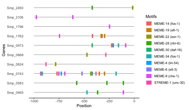
p.st1<-ggplot(data = top10markers, aes(gene, -1000)) + geom_bar(stat="identity", fill="grey", width = 0.05, height=1000, position = position_stack(reverse = TRUE)) +coord_flip()+labs(x="Genes", y="Position")+ylim(-1000,0)
# now add segments as the motifs
p.st1<-p.st1+geom_segment(data=top10markers, aes(x=gene, xend=gene, y=start*(-1), yend=stop*(-1), color=jaspar), size=5)
# change legend title and remove y-axis
p.st1<-p.st1+theme_classic()+labs(color="Motifs")+theme(axis.ticks.y = element_blank(),, axis.line.y = element_blank())
p.st1
|
The above example is to visualise all different sub-features on the same gene. Another situation is to visualise different genes with the same feature (such as protein domain).
For instance I have a list of clusters within which all genes have the same Pfam, and another file with information about the positions of matched Pfam, as well as length and coordinates of the peptides.
 1
 2
 3
 4
 5
 6
 7
 8
 9
10
11
12
13
|
# information of the clusters
sample_n(allClusters, 2)

       chr    Pfam         pf_name                    description gene_counts
1  SM_V7_1 PF01221    Dynein_light     Dynein_light_chain_type_1_           7
2 SM_V7_ZW PF17039 Glyco_tran_10_N Fucosyltransferase,_N-terminal           3

# information on peptides and pfam domains
sample_n(pfamInfo, 2)

            id     chr    start strand pep_len    Pfam pf_start pf_end
1 Smp_162630.1 SM_V7_3 20366872      -    1058 PF16191      293    361
2 Smp_159600.2 SM_V7_1  9907913      -    1762 PF01391      720    773
|
So the idea is to visualise each cluster, where all peptides with their matched pfam features will be shown.
 1
 2
 3
 4
 5
 6
 7
 8
 9
10
11
12
13
14
15
|
# select a cluster
cluster1<-allClusters[49,]

# get all transcripts and pfam domains in that clusters
cluster1.range<-pfamInfo[which(as.character(cluster1$chr)==as.character(pfamInfo$chr) & pfamInfo$start >= cluster1$first_start & pfamInfo$start <= cluster1$last_start & as.character(cluster1$Pfam)==as.character(pfamInfo$Pfam)),]

cluster1.range

                id     chr    start strand pep_len    Pfam pf_start pf_end
14417 Smp_344710.1 SM_V7_5 20379409      +     498 PF09728       34    334
14418 Smp_332120.1 SM_V7_5 20465519      +     299 PF09728        5     83
14419 Smp_330720.1 SM_V7_5 20484109      +     361 PF09728       45    159
14420 Smp_332130.1 SM_V7_5 20519729      +     778 PF09728      329    443
14421 Smp_332130.1 SM_V7_5 20519729      +     778 PF09728      495    617
14422 Smp_332130.1 SM_V7_5 20519729      +     778 PF09728        5    124
|
Now to draw the features
1
2
3
4
5
|
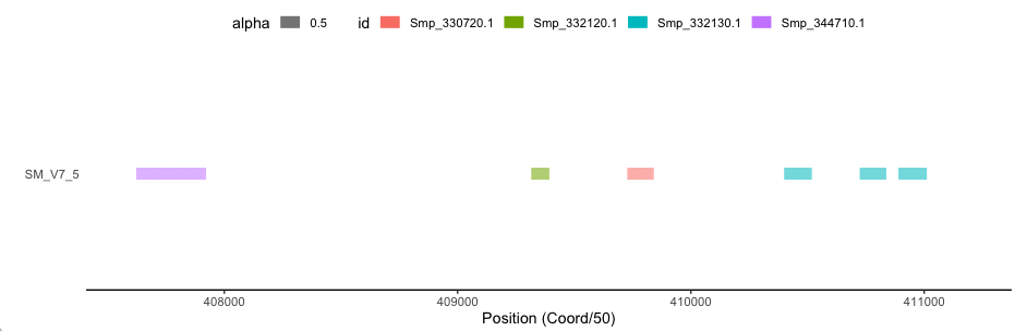
# limit the range of genomic bar
ps<-ggplot(data=cluster1.range, aes(chr, 10000)) +  geom_bar(stat="identity", fill="grey", width = 0.05, position = position_stack(reverse = TRUE)) +coord_flip()+labs(x="", y="Position (Coord/50)")+ylim(min(cluster1.range$start)/50, max(cluster1.range$start)/50+800)

# add Pfam segments
ps1<-ps+geom_segment(data=cluster1.range, aes(x=chr, xend=chr, y=start/50+pf_start, yend=start/50+pf_end, color=id, alpha = 0.5), size=4)+theme_classic()+theme(axis.ticks.y = element_blank(),axis.line.y = element_blank())+theme(legend.position = "top")
|
1
2
3
4
5
6
7
8
9
|
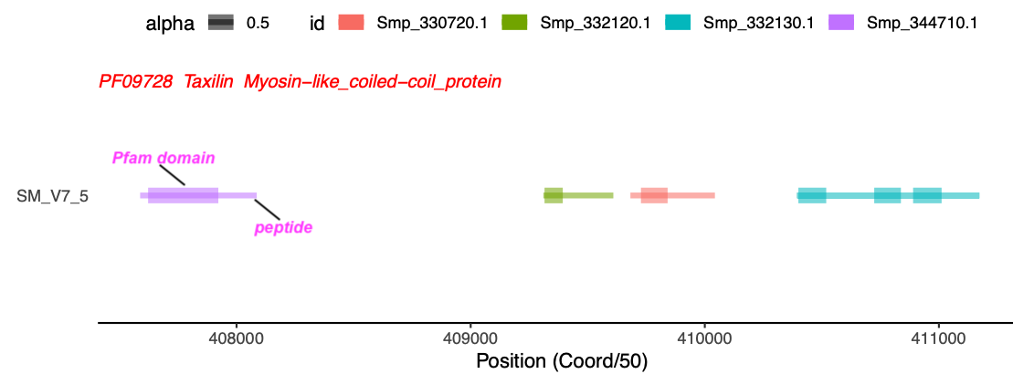
# add peptide segments
ps2<-ps1+geom_segment(data=cluster1.range, aes(x=chr, xend=chr, y=start/50, yend=start/50+pep_len, colour=id, alpha=0.5), size=1.5)

library(grid)
# Create a text
grob <- grobTree(textGrob(paste(cluster1$Pfam, cluster1$pf_name, cluster1$description, sep="  "), x=0,  y=0.95, hjust=0, gp=gpar(col="red", fontsize=10, fontface="italic")))

# add text to the plot
ps2<-ps2 +annotation_custom(grob)
|